TÄNA AJALOOS, 24. juuli ⟩ Ameerika professor leidis mägedest maailmakuulsa hüljatud linna

Unsupervised learning is a framework in machine learning where, in contrast to supervised learning, algorithms learn patterns exclusively from unlabeled data.^[1] Other frameworks in the spectrum of supervisions include weak- or semi-supervision, where a small portion of the data is tagged, and self-supervision. Some researchers consider self-supervised learning a form of unsupervised learning.^[2]

Conceptually, unsupervised learning divides into the aspects of data, training, algorithm, and downstream applications. Typically, the dataset is harvested cheaply "in the wild", such as massive text corpus obtained by web crawling, with only minor filtering (such as Common Crawl). This compares favorably to supervised learning, where the dataset (such as the ImageNet1000) is typically constructed manually, which is much more expensive.

There are algorithms designed specifically for unsupervised learning, such as clustering algorithms like k-means, dimensionality reduction techniques like principal component analysis (PCA), Boltzmann machine learning, and autoencoders. After the rise of deep learning, most large-scale unsupervised learning has been done by training general-purpose neural network architectures by gradient descent, adapted to performing unsupervised learning by designing an appropriate training procedure.

Sometimes a trained model can be used as-is, but more often they are modified for downstream applications. For example, the generative pretraining method trains a model to generate a textual dataset, before finetuning it for other applications, such as text classification.^[3]^[4] As another example, autoencoders are trained to produce good features, which can then be used as a module for other models, such as in a latent diffusion model.

Tasks

Tendency for a task to employ supervised vs. unsupervised methods. Task names straddling circle boundaries is intentional. It shows that the classical division of imaginative tasks (left) employing unsupervised methods is blurred in today's learning schemes.

Tasks are often categorized as discriminative (recognition) or generative (imagination). Often but not always, discriminative tasks use supervised methods and generative tasks use unsupervised (see Venn diagram); however, the separation is very hazy. For example, object recognition favors supervised learning but unsupervised learning can also cluster objects into groups. Furthermore, as progress marches onward, some tasks employ both methods, and some tasks swing from one to another. For example, image recognition started off as heavily supervised, but became hybrid by employing unsupervised pre-training, and then moved towards supervision again with the advent of dropout, ReLU, and adaptive learning rates.

A typical generative task is as follows. At each step, a datapoint is sampled from the dataset, and part of the data is removed, and the model must infer the removed part. This is particularly clear for the denoising autoencoders and BERT.

Neural network architectures

Training

During the learning phase, an unsupervised network tries to mimic the data it is given and uses the error in its mimicked output to correct itself (i.e. correct its weights and biases). Sometimes the error is expressed as a low probability that the erroneous output occurs, or it might be expressed as an unstable high energy state in the network.

In contrast to supervised methods' dominant use of backpropagation, unsupervised learning also employs other methods including: Hopfield learning rule, Boltzmann learning rule, Contrastive Divergence, Wake Sleep, Variational Inference, Maximum Likelihood, Maximum A Posteriori, Gibbs Sampling, and backpropagating reconstruction errors or hidden state reparameterizations. See the table below for more details.

Energy

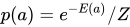
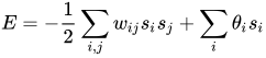
An energy function is a macroscopic measure of a network's activation state. In Boltzmann machines, it plays the role of the Cost function. This analogy with physics is inspired by Ludwig Boltzmann's analysis of a gas' macroscopic energy from the microscopic probabilities of particle motion $p\propto e^{-E/kT}$ , where k is the Boltzmann constant and T is temperature. In the RBM network the relation is $p=e^{-E}/Z$ ,^[5] where $p$ and $E$ vary over every possible activation pattern and $\textstyle {Z=\sum _{\scriptscriptstyle {\text{All Patterns}}}e^{-E({\text{pattern}})}}$ . To be more precise, $p(a)=e^{-E(a)}/Z$ , where $a$ is an activation pattern of all neurons (visible and hidden). Hence, some early neural networks bear the name Boltzmann Machine. Paul Smolensky calls $-E\,$ the Harmony. A network seeks low energy which is high Harmony.

Networks

This table shows connection diagrams of various unsupervised networks, the details of which will be given in the section Comparison of Networks. Circles are neurons and edges between them are connection weights. As network design changes, features are added on to enable new capabilities or removed to make learning faster. For instance, neurons change between deterministic (Hopfield) and stochastic (Boltzmann) to allow robust output, weights are removed within a layer (RBM) to hasten learning, or connections are allowed to become asymmetric (Helmholtz).

Hopfield	Boltzmann	RBM	Stacked Boltzmann
A network based on magnetic domains in iron with a single self-connected layer. It can be used as a content addressable memory.	Network is separated into 2 layers (hidden vs. visible), but still using symmetric 2-way weights. Following Boltzmann's thermodynamics, individual probabilities give rise to macroscopic energies.	Restricted Boltzmann Machine. This is a Boltzmann machine where lateral connections within a layer are prohibited to make analysis tractable.	This network has multiple RBM's to encode a hierarchy of hidden features. After a single RBM is trained, another blue hidden layer (see left RBM) is added, and the top 2 layers are trained as a red & blue RBM. Thus the middle layers of an RBM acts as hidden or visible, depending on the training phase it is in.

Helmholtz	Autoencoder	VAE
Instead of the bidirectional symmetric connection of the stacked Boltzmann machines, we have separate one-way connections to form a loop. It does both generation and discrimination.	A feed forward network that aims to find a good middle layer representation of its input world. This network is deterministic, so it is not as robust as its successor the VAE.	Applies Variational Inference to the Autoencoder. The middle layer is a set of means & variances for Gaussian distributions. The stochastic nature allows for more robust imagination than the deterministic autoencoder.

Of the networks bearing people's names, only Hopfield worked directly with neural networks. Boltzmann and Helmholtz came before artificial neural networks, but their work in physics and physiology inspired the analytical methods that were used.

History

1974	Ising magnetic model proposed by WA Little [de] for cognition
1980	Kunihiko Fukushima introduces the neocognitron, which is later called a convolutional neural network. It is mostly used in SL, but deserves a mention here.
1982	Ising variant Hopfield net described as CAMs and classifiers by John Hopfield.
1983	Ising variant Boltzmann machine with probabilistic neurons described by Hinton & Sejnowski following Sherington & Kirkpatrick's 1975 work.
1986	Paul Smolensky publishes Harmony Theory, which is an RBM with practically the same Boltzmann energy function. Smolensky did not give a practical training scheme. Hinton did in mid-2000s.
1995	Hochreiter and Schmidhuber introduce the LSTM neuron for languages.
1995	Dayan & Hinton introduces Helmholtz machine
2013	Kingma, Rezende, & co. introduced Variational Autoencoders as Bayesian graphical probability network, with neural nets as components.

Specific networks

Here, we highlight some characteristics of select networks. The details of each are given in the comparison table below.

Comparison of networks

	Hopfield	Boltzmann	RBM	Stacked RBM	Helmholtz	Autoencoder	VAE
Usage & notables	CAM, traveling salesman problem	CAM. The freedom of connections makes this network difficult to analyze.	pattern recognition. used in MNIST digits and speech.	recognition & imagination. trained with unsupervised pre-training and/or supervised fine tuning.	imagination, mimicry	language: creative writing, translation. vision: enhancing blurry images	generate realistic data
Neuron	deterministic binary state. Activation = { 0 (or -1) if x is negative, 1 otherwise }	stochastic binary Hopfield neuron	← same. (extended to real-valued in mid 2000s)	← same	← same	language: LSTM. vision: local receptive fields. usually real valued relu activation.	middle layer neurons encode means & variances for Gaussians. In run mode (inference), the output of the middle layer are sampled values from the Gaussians.
Connections	1-layer with symmetric weights. No self-connections.	2-layers. 1-hidden & 1-visible. symmetric weights.	← same. no lateral connections within a layer.	top layer is undirected, symmetric. other layers are 2-way, asymmetric.	3-layers: asymmetric weights. 2 networks combined into 1.	3-layers. The input is considered a layer even though it has no inbound weights. recurrent layers for NLP. feedforward convolutions for vision. input & output have the same neuron counts.	3-layers: input, encoder, distribution sampler decoder. the sampler is not considered a layer
Inference & energy	Energy is given by Gibbs probability measure : $E=-{\frac {1}{2}}\sum _{i,j}{w_{ij}{s_{i}}{s_{j}}}+\sum _{i}{\theta _{i}}{s_{i}}$	← same	← same		minimize KL divergence	inference is only feed-forward. previous UL networks ran forwards AND backwards	minimize error = reconstruction error - KLD
Training	Δw_ij = s_i*s_j, for +1/-1 neuron	Δw_ij = e*(p_ij - p'_ij). This is derived from minimizing KLD. e = learning rate, p' = predicted and p = actual distribution.	Δw_ij = e*( < v_i h_j >_data - < v_i h_j >_equilibrium ). This is a form of contrastive divergence w/ Gibbs Sampling. "<>" are expectations.	← similar. train 1-layer at a time. approximate equilibrium state with a 3-segment pass. no back propagation.	wake-sleep 2 phase training	back propagate the reconstruction error	reparameterize hidden state for backprop
Strength	resembles physical systems so it inherits their equations	← same. hidden neurons act as internal representatation of the external world	faster more practical training scheme than Boltzmann machines	trains quickly. gives hierarchical layer of features	mildly anatomical. analyzable w/ information theory & statistical mechanics
Weakness		hard to train due to lateral connections	equilibrium requires too many iterations	integer & real-valued neurons are more complicated.

Hebbian Learning, ART, SOM

The classical example of unsupervised learning in the study of neural networks is Donald Hebb's principle, that is, neurons that fire together wire together.^[8] In Hebbian learning, the connection is reinforced irrespective of an error, but is exclusively a function of the coincidence between action potentials between the two neurons.^[9] A similar version that modifies synaptic weights takes into account the time between the action potentials (spike-timing-dependent plasticity or STDP). Hebbian Learning has been hypothesized to underlie a range of cognitive functions, such as pattern recognition and experiential learning.

Among neural network models, the self-organizing map (SOM) and adaptive resonance theory (ART) are commonly used in unsupervised learning algorithms. The SOM is a topographic organization in which nearby locations in the map represent inputs with similar properties. The ART model allows the number of clusters to vary with problem size and lets the user control the degree of similarity between members of the same clusters by means of a user-defined constant called the vigilance parameter. ART networks are used for many pattern recognition tasks, such as automatic target recognition and seismic signal processing.^[10]

Probabilistic methods

Two of the main methods used in unsupervised learning are principal component and cluster analysis. Cluster analysis is used in unsupervised learning to group, or segment, datasets with shared attributes in order to extrapolate algorithmic relationships.^[11] Cluster analysis is a branch of machine learning that groups the data that has not been labelled, classified or categorized. Instead of responding to feedback, cluster analysis identifies commonalities in the data and reacts based on the presence or absence of such commonalities in each new piece of data. This approach helps detect anomalous data points that do not fit into either group.

A central application of unsupervised learning is in the field of density estimation in statistics,^[12] though unsupervised learning encompasses many other domains involving summarizing and explaining data features. It can be contrasted with supervised learning by saying that whereas supervised learning intends to infer a conditional probability distribution conditioned on the label of input data; unsupervised learning intends to infer an a priori probability distribution .

Approaches

Some of the most common algorithms used in unsupervised learning include: (1) Clustering, (2) Anomaly detection, (3) Approaches for learning latent variable models. Each approach uses several methods as follows:

Clustering methods include: hierarchical clustering,^[13] k-means,^[14] mixture models, model-based clustering, DBSCAN, and OPTICS algorithm
Anomaly detection methods include: local outlier factor, and isolation forest
Approaches for learning latent variable models such as expectation–maximization algorithm (EM), method of moments, and blind signal separation techniques (principal component analysis, independent component analysis, non-negative matrix factorization, singular value decomposition)

Method of moments

One of the statistical approaches for unsupervised learning is the method of moments. In the method of moments, the unknown parameters (of interest) in the model are related to the moments of one or more random variables, and thus, these unknown parameters can be estimated given the moments. The moments are usually estimated from samples empirically. The basic moments are first and second order moments. For a random vector, the first order moment is the mean vector, and the second order moment is the covariance matrix (when the mean is zero). Higher order moments are usually represented using tensors which are the generalization of matrices to higher orders as multi-dimensional arrays.

In particular, the method of moments is shown to be effective in learning the parameters of latent variable models. Latent variable models are statistical models where in addition to the observed variables, a set of latent variables also exists which is not observed. A highly practical example of latent variable models in machine learning is the topic modeling which is a statistical model for generating the words (observed variables) in the document based on the topic (latent variable) of the document. In the topic modeling, the words in the document are generated according to different statistical parameters when the topic of the document is changed. It is shown that method of moments (tensor decomposition techniques) consistently recover the parameters of a large class of latent variable models under some assumptions.^[15]

The Expectation–maximization algorithm (EM) is also one of the most practical methods for learning latent variable models. However, it can get stuck in local optima, and it is not guaranteed that the algorithm will converge to the true unknown parameters of the model. In contrast, for the method of moments, the global convergence is guaranteed under some conditions.

References

↑ Wu, Wei. "Unsupervised Learning" (PDF). Archived (PDF) from the original on 14 April 2024. Retrieved 26 April 2024.
↑ Liu, Xiao; Zhang, Fanjin; Hou, Zhenyu; Mian, Li; Wang, Zhaoyu; Zhang, Jing; Tang, Jie (2021). "Self-supervised Learning: Generative or Contrastive". IEEE Transactions on Knowledge and Data Engineering: 1. arXiv:2006.08218. doi:10.1109/TKDE.2021.3090866. ISSN 1041-4347.
↑ Radford, Alec; Narasimhan, Karthik; Salimans, Tim; Sutskever, Ilya (11 June 2018). "Improving Language Understanding by Generative Pre-Training" (PDF). OpenAI. p. 12. Archived (PDF) from the original on 26 January 2021. Retrieved 23 January 2021.
↑ Li, Zhuohan; Wallace, Eric; Shen, Sheng; Lin, Kevin; Keutzer, Kurt; Klein, Dan; Gonzalez, Joey (2020-11-21). "Train Big, Then Compress: Rethinking Model Size for Efficient Training and Inference of Transformers". Proceedings of the 37th International Conference on Machine Learning. PMLR: 5958–5968.
↑ Hinton, G. (2012). "A Practical Guide to Training Restricted Boltzmann Machines" (PDF). Neural Networks: Tricks of the Trade. Lecture Notes in Computer Science. Vol. 7700. Springer. pp. 599–619. doi:10.1007/978-3-642-35289-8_32. ISBN 978-3-642-35289-8. Archived (PDF) from the original on 2022-09-03. Retrieved 2022-11-03.
↑ "Deep Belief Nets" (video). September 2009. Archived from the original on 2022-03-08. Retrieved 2022-03-27.
↑ Peter, Dayan; Hinton, Geoffrey E.; Neal, Radford M.; Zemel, Richard S. (1995). "The Helmholtz machine". Neural Computation. 7 (5): 889–904. doi:10.1162/neco.1995.7.5.889. hdl:21.11116/0000-0002-D6D3-E. PMID 7584891. S2CID 1890561.
↑ Buhmann, J.; Kuhnel, H. (1992). "Unsupervised and supervised data clustering with competitive neural networks". [Proceedings 1992] IJCNN International Joint Conference on Neural Networks. Vol. 4. IEEE. pp. 796–801. doi:10.1109/ijcnn.1992.227220. ISBN 0780305590. S2CID 62651220.
↑ Comesaña-Campos, Alberto; Bouza-Rodríguez, José Benito (June 2016). "An application of Hebbian learning in the design process decision-making". Journal of Intelligent Manufacturing. 27 (3): 487–506. doi:10.1007/s10845-014-0881-z. ISSN 0956-5515. S2CID 207171436.
↑ Carpenter, G.A. & Grossberg, S. (1988). "The ART of adaptive pattern recognition by a self-organizing neural network" (PDF). Computer. 21 (3): 77–88. doi:10.1109/2.33. S2CID 14625094. Archived from the original (PDF) on 2018-05-16. Retrieved 2013-09-16.
↑ Roman, Victor (2019-04-21). "Unsupervised Machine Learning: Clustering Analysis". Medium. Archived from the original on 2020-08-21. Retrieved 2019-10-01.
↑ Jordan, Michael I.; Bishop, Christopher M. (2004). "7. Intelligent Systems §Neural Networks". In Tucker, Allen B. (ed.). Computer Science Handbook (2nd ed.). Chapman & Hall/CRC Press. doi:10.1201/9780203494455. ISBN 1-58488-360-X. Archived from the original on 2022-11-03. Retrieved 2022-11-03.
↑ Hastie, Tibshirani & Friedman 2009, pp. 485–586
↑ Garbade, Dr Michael J. (2018-09-12). "Understanding K-means Clustering in Machine Learning". Medium. Archived from the original on 2019-05-28. Retrieved 2019-10-31.
↑ Anandkumar, Animashree; Ge, Rong; Hsu, Daniel; Kakade, Sham; Telgarsky, Matus (2014). "Tensor Decompositions for Learning Latent Variable Models" (PDF). Journal of Machine Learning Research. 15: 2773–2832. arXiv:1210.7559. Bibcode:2012arXiv1210.7559A. Archived (PDF) from the original on 2015-03-20. Retrieved 2015-04-10.

Differentiable computing
General	Differentiable programming Information geometry Statistical manifold Automatic differentiation Neuromorphic computing Pattern recognition Ricci calculus Computational learning theory Inductive bias
Hardware	IPU TPU VPU Memristor SpiNNaker
Software libraries	TensorFlow PyTorch Keras scikit-learn Theano JAX Flux.jl MindSpore
Portals Computer programming Technology

TÄNA AJALOOS, 24. juuli ⟩ Ameerika professor leidis mägedest maailmakuulsa hüljatud linna

Tasks