
In probability theory and statistics, the multivariate normal distribution, multivariate Gaussian distribution, or joint normal distribution is a generalization of the one-dimensional (univariate) normal distribution to higher dimensions. One definition is that a random vector is said to be k-variate normally distributed if every linear combination of its k components has a univariate normal distribution. Its importance derives mainly from the multivariate central limit theorem. The multivariate normal distribution is often used to describe, at least approximately, any set of (possibly) correlated real-valued random variables, each of which clusters around a mean value.
Definitions
Notation and parametrization
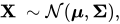
The multivariate normal distribution of a k-dimensional random vector can be written in the following notation:


or to make it explicitly known that is k-dimensional,


with k-dimensional mean vector
![{\displaystyle {\boldsymbol {\mu }}=\operatorname {E} [\mathbf {X} ]=(\operatorname {E} [X_{1}],\operatorname {E} [X_{2}],\ldots ,\operatorname {E} [X_{k}])^{\mathrm {T} },}](https://wikimedia.org/api/rest_v1/media/math/render/svg/a0ff77227bef5ec255a816fbb1a31d5c1e0fba21)

![{\displaystyle \Sigma _{i,j}=\operatorname {E} [(X_{i}-\mu _{i})(X_{j}-\mu _{j})]=\operatorname {Cov} [X_{i},X_{j}]}](https://wikimedia.org/api/rest_v1/media/math/render/svg/c970083f8469366521881996464f23d376b7c40b)
such that and . The inverse of the covariance matrix is called the precision matrix, denoted by .


Standard normal random vector
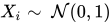
A real random vector is called a standard normal random vector if all of its components are independent and each is a zero-mean unit-variance normally distributed random variable, i.e. if for all .[1]: p. 454


Centered normal random vector
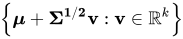
A real random vector is called a centered normal random vector if there exists a matrix such that has the same distribution as where is a standard normal random vector with components.[1]: p. 454


Normal random vector
A real random vector is called a normal random vector if there exists a random -vector , which is a standard normal random vector, a -vector , and a matrix , such that .[2]: p. 454 [1]: p. 455


Formally:

Here the covariance matrix is .

In the degenerate case where the covariance matrix is singular, the corresponding distribution has no density; see the section below for details. This case arises frequently in statistics; for example, in the distribution of the vector of residuals in the ordinary least squares regression. The are in general not independent; they can be seen as the result of applying the matrix to a collection of independent Gaussian variables .
Equivalent definitions
The following definitions are equivalent to the definition given above. A random vector has a multivariate normal distribution if it satisfies one of the following equivalent conditions.
- Every linear combination of its components is normally distributed. That is, for any constant vector , the random variable has a univariate normal distribution, where a univariate normal distribution with zero variance is a point mass on its mean.
- There is a k-vector and a symmetric, positive semidefinite matrix , such that the characteristic function of is




The spherical normal distribution can be characterised as the unique distribution where components are independent in any orthogonal coordinate system.[3][4]
Density function

Non-degenerate case
The multivariate normal distribution is said to be "non-degenerate" when the symmetric covariance matrix is positive definite. In this case the distribution has density[5]

where is a real k-dimensional column vector and is the determinant of , also known as the generalized variance. The subexpression can be re-written as , which is especially useful in the degenerate case; see below. The equation above reduces to that of the univariate normal distribution if is a matrix (i.e., a single real number).


The circularly symmetric version of the complex normal distribution has a slightly different form.
Each iso-density locus — the locus of points in k-dimensional space each of which gives the same particular value of the density — is an ellipse or its higher-dimensional generalization; hence the multivariate normal is a special case of the elliptical distributions.
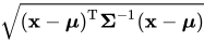
The quantity is known as the Mahalanobis distance, which represents the distance of the test point from the mean . The squared Mahalanobis distance is decomposed into a sum of k terms, each term being a product of three meaningful components.[6] Note that in the case when , the distribution reduces to a univariate normal distribution and the Mahalanobis distance reduces to the absolute value of the standard score. See also Interval below.


Bivariate case
In the 2-dimensional nonsingular case (), the probability density function of a vector is: where is the correlation between and and where and . In this case,

![{\displaystyle {\text{[XY]}}\prime }](https://wikimedia.org/api/rest_v1/media/math/render/svg/faffc663dc20d1db9845a496c725e6b07029f263)
![{\displaystyle f(x,y)={\frac {1}{2\pi \sigma _{X}\sigma _{Y}{\sqrt {1-\rho ^{2}}}}}\exp \left(-{\frac {1}{2\left[1-\rho ^{2}\right]}}\left[\left({\frac {x-\mu _{X}}{\sigma _{X}}}\right)^{2}-2\rho \left({\frac {x-\mu _{X}}{\sigma _{X}}}\right)\left({\frac {y-\mu _{Y}}{\sigma _{Y}}}\right)+\left({\frac {y-\mu _{Y}}{\sigma _{Y}}}\right)^{2}\right]\right)}](https://wikimedia.org/api/rest_v1/media/math/render/svg/bf91aebe806d84bb97ab95715e8e10e619387356)



In the bivariate case, the first equivalent condition for multivariate reconstruction of normality can be made less restrictive as it is sufficient to verify that a countably infinite set of distinct linear combinations of and are normal in order to conclude that the vector of is bivariate normal.[7]
The bivariate iso-density loci plotted in the -plane are ellipses, whose principal axes are defined by the eigenvectors of the covariance matrix (the major and minor semidiameters of the ellipse equal the square-root of the ordered eigenvalues).


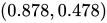
As the absolute value of the correlation parameter increases, these loci are squeezed toward the following line :

This is because this expression, with (where sgn is the sign function) replaced by , is the best linear unbiased prediction of given a value of .[8]

Degenerate case
If the covariance matrix is not full rank, then the multivariate normal distribution is degenerate and does not have a density. More precisely, it does not have a density with respect to k-dimensional Lebesgue measure (which is the usual measure assumed in calculus-level probability courses). Only random vectors whose distributions are absolutely continuous with respect to a measure are said to have densities (with respect to that measure). To talk about densities but avoid dealing with measure-theoretic complications it can be simpler to restrict attention to a subset of of the coordinates of such that the covariance matrix for this subset is positive definite; then the other coordinates may be thought of as an affine function of these selected coordinates.[9]


To talk about densities meaningfully in singular cases, then, we must select a different base measure. Using the disintegration theorem we can define a restriction of Lebesgue measure to the -dimensional affine subspace of where the Gaussian distribution is supported, i.e. . With respect to this measure the distribution has the density of the following motif:

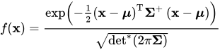
where is the generalized inverse and is the pseudo-determinant.[10]


Cumulative distribution function
The notion of cumulative distribution function (cdf) in dimension 1 can be extended in two ways to the multidimensional case, based on rectangular and ellipsoidal regions.
The first way is to define the cdf of a random vector as the probability that all components of are less than or equal to the corresponding values in the vector :[11]


Though there is no closed form for , there are a number of algorithms that estimate it numerically.[11][12]
Another way is to define the cdf as the probability that a sample lies inside the ellipsoid determined by its Mahalanobis distance from the Gaussian, a direct generalization of the standard deviation.[13] In order to compute the values of this function, closed analytic formula exist,[13] as follows.


Interval
The interval for the multivariate normal distribution yields a region consisting of those vectors x satisfying

Here is a -dimensional vector, is the known -dimensional mean vector, is the known covariance matrix and is the quantile function for probability of the chi-squared distribution with degrees of freedom.[14] When the expression defines the interior of an ellipse and the chi-squared distribution simplifies to an exponential distribution with mean equal to two (rate equal to half).


Complementary cumulative distribution function (tail distribution)
The complementary cumulative distribution function (ccdf) or the tail distribution is defined as . When , then the ccdf can be written as a probability the maximum of dependent Gaussian variables:[15]

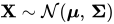

While no simple closed formula exists for computing the ccdf, the maximum of dependent Gaussian variables can be estimated accurately via the Monte Carlo method.[15][16]
Properties
Moments
The kth-order moments of x are given by
![{\displaystyle \mu _{1,\ldots ,N}(\mathbf {x} )\mathrel {\stackrel {\mathrm {def} }{=}} \mu _{r_{1},\ldots ,r_{N}}(\mathbf {x} )\mathrel {\stackrel {\mathrm {def} }{=}} \operatorname {E} \left[\prod _{j=1}^{N}X_{j}^{r_{j}}\right]}](https://wikimedia.org/api/rest_v1/media/math/render/svg/e19f7eec8adb98477e74dd88285ec1a07ce29aef)
where
where the sum is taken over all allocations of the set into λ (unordered) pairs. That is, for a kth (= 2λ = 6) central moment, one sums the products of λ = 3 covariances (the expected value μ is taken to be 0 in the interests of parsimony):

![{\displaystyle {\begin{aligned}&\operatorname {E} [X_{1}X_{2}X_{3}X_{4}X_{5}X_{6}]\\[8pt]={}&\operatorname {E} [X_{1}X_{2}]\operatorname {E} [X_{3}X_{4}]\operatorname {E} [X_{5}X_{6}]+\operatorname {E} [X_{1}X_{2}]\operatorname {E} [X_{3}X_{5}]\operatorname {E} [X_{4}X_{6}]+\operatorname {E} [X_{1}X_{2}]\operatorname {E} [X_{3}X_{6}]\operatorname {E} [X_{4}X_{5}]\\[4pt]&{}+\operatorname {E} [X_{1}X_{3}]\operatorname {E} [X_{2}X_{4}]\operatorname {E} [X_{5}X_{6}]+\operatorname {E} [X_{1}X_{3}]\operatorname {E} [X_{2}X_{5}]\operatorname {E} [X_{4}X_{6}]+\operatorname {E} [X_{1}X_{3}]\operatorname {E} [X_{2}X_{6}]\operatorname {E} [X_{4}X_{5}]\\[4pt]&{}+\operatorname {E} [X_{1}X_{4}]\operatorname {E} [X_{2}X_{3}]\operatorname {E} [X_{5}X_{6}]+\operatorname {E} [X_{1}X_{4}]\operatorname {E} [X_{2}X_{5}]\operatorname {E} [X_{3}X_{6}]+\operatorname {E} [X_{1}X_{4}]\operatorname {E} [X_{2}X_{6}]\operatorname {E} [X_{3}X_{5}]\\[4pt]&{}+\operatorname {E} [X_{1}X_{5}]\operatorname {E} [X_{2}X_{3}]\operatorname {E} [X_{4}X_{6}]+\operatorname {E} [X_{1}X_{5}]\operatorname {E} [X_{2}X_{4}]\operatorname {E} [X_{3}X_{6}]+\operatorname {E} [X_{1}X_{5}]\operatorname {E} [X_{2}X_{6}]\operatorname {E} [X_{3}X_{4}]\\[4pt]&{}+\operatorname {E} [X_{1}X_{6}]\operatorname {E} [X_{2}X_{3}]\operatorname {E} [X_{4}X_{5}]+\operatorname {E} [X_{1}X_{6}]\operatorname {E} [X_{2}X_{4}]\operatorname {E} [X_{3}X_{5}]+\operatorname {E} [X_{1}X_{6}]\operatorname {E} [X_{2}X_{5}]\operatorname {E} [X_{3}X_{4}].\end{aligned}}}](https://wikimedia.org/api/rest_v1/media/math/render/svg/0517839a9528128fa6d69cedfe4f5003a34716f4)
This yields terms in the sum (15 in the above case), each being the product of λ (in this case 3) covariances. For fourth order moments (four variables) there are three terms. For sixth-order moments there are 3 × 5 = 15 terms, and for eighth-order moments there are 3 × 5 × 7 = 105 terms.

The covariances are then determined by replacing the terms of the list by the corresponding terms of the list consisting of r1 ones, then r2 twos, etc.. To illustrate this, examine the following 4th-order central moment case:
![{\displaystyle [1,\ldots ,2\lambda ]}](https://wikimedia.org/api/rest_v1/media/math/render/svg/a605bf32a38577fe9df1bc5715a4a3cac5869832)
![{\displaystyle {\begin{aligned}\operatorname {E} \left[X_{i}^{4}\right]&=3\sigma _{ii}^{2}\\[4pt]\operatorname {E} \left[X_{i}^{3}X_{j}\right]&=3\sigma _{ii}\sigma _{ij}\\[4pt]\operatorname {E} \left[X_{i}^{2}X_{j}^{2}\right]&=\sigma _{ii}\sigma _{jj}+2\sigma _{ij}^{2}\\[4pt]\operatorname {E} \left[X_{i}^{2}X_{j}X_{k}\right]&=\sigma _{ii}\sigma _{jk}+2\sigma _{ij}\sigma _{ik}\\[4pt]\operatorname {E} \left[X_{i}X_{j}X_{k}X_{n}\right]&=\sigma _{ij}\sigma _{kn}+\sigma _{ik}\sigma _{jn}+\sigma _{in}\sigma _{jk}.\end{aligned}}}](https://wikimedia.org/api/rest_v1/media/math/render/svg/4e08f5bc180e3f1f4379c1026100e833ea85de97)
where is the covariance of Xi and Xj. With the above method one first finds the general case for a kth moment with k different X variables, , and then one simplifies this accordingly. For example, for , one lets Xi = Xj and one uses the fact that .

![{\displaystyle E\left[X_{i}X_{j}X_{k}X_{n}\right]}](https://wikimedia.org/api/rest_v1/media/math/render/svg/0b4bbbf2becaf15b246898e928a37e7d0ab6f93a)
![{\displaystyle \operatorname {E} [X_{i}^{2}X_{k}X_{n}]}](https://wikimedia.org/api/rest_v1/media/math/render/svg/f7bc1920d0e524aa567ca471bdb54dcf7ef7e673)

Functions of a normal vector
A quadratic form of a normal vector , (where is a matrix, is a vector, and is a scalar), is a generalized chi-squared variable. The direction of a normal vector follows a projected normal distribution.[17]




If is a general scalar-valued function of a normal vector, its probability density function, cumulative distribution function, and inverse cumulative distribution function can be computed with the numerical method of ray-tracing (Matlab code Archived 2025-02-20 at the Wayback Machine).

Likelihood function
If the mean and covariance matrix are known, the log likelihood of an observed vector is simply the log of the probability density function:
- ,
![{\displaystyle \ln L({\boldsymbol {x}})=-{\frac {1}{2}}\left[\ln(|{\boldsymbol {\Sigma }}|\,)+({\boldsymbol {x}}-{\boldsymbol {\mu }})'{\boldsymbol {\Sigma }}^{-1}({\boldsymbol {x}}-{\boldsymbol {\mu }})+k\ln(2\pi )\right]}](https://wikimedia.org/api/rest_v1/media/math/render/svg/4ad05643016bbf6ac76a826320bea00704b50982)
The circularly symmetric version of the noncentral complex case, where is a vector of complex numbers, would be


i.e. with the conjugate transpose (indicated by ) replacing the normal transpose (indicated by ). This is slightly different than in the real case, because the circularly symmetric version of the complex normal distribution has a slightly different form for the normalization constant.


A similar notation is used for multiple linear regression.[18]
Since the log likelihood of a normal vector is a quadratic form of the normal vector, it is distributed as a generalized chi-squared variable.
Differential entropy
The differential entropy of the multivariate normal distribution is[19]
![{\displaystyle {\begin{aligned}h\left(f\right)&=-\int _{-\infty }^{\infty }\int _{-\infty }^{\infty }\cdots \int _{-\infty }^{\infty }f(\mathbf {x} )\ln f(\mathbf {x} )\,d\mathbf {x} \\[1ex]&={\frac {1}{2}}\ln \left|2\pi e{\boldsymbol {\Sigma }}\right|={\frac {k}{2}}\left(1+\ln 2\pi \right)+{\frac {1}{2}}\ln \left|{\boldsymbol {\Sigma }}\right|,\end{aligned}}}](https://wikimedia.org/api/rest_v1/media/math/render/svg/c58f166409e0c1adef2a3a48f1a60f1119697cbe)
where the bars denote the matrix determinant, k is the dimensionality of the vector space, and the result has units of nats.
Kullback–Leibler divergence
The Kullback–Leibler divergence from to , for non-singular matrices Σ1 and Σ0, is:[20]



where denotes the matrix determinant, is the trace, is the natural logarithm and is the dimension of the vector space.


The logarithm must be taken to base e since the two terms following the logarithm are themselves base-e logarithms of expressions that are either factors of the density function or otherwise arise naturally. The equation therefore gives a result measured in nats. Dividing the entire expression above by loge 2 yields the divergence in bits.
When ,


Mutual information
The mutual information of two multivariate normal distribution is a special case of the Kullback–Leibler divergence in which is the full dimensional multivariate distribution and is the product of the and dimensional marginal distributions and , such that . The mutual information between and is given by:[21]


where

If is product of one-dimensional normal distributions, then in the notation of the Kullback–Leibler divergence section of this article, is a diagonal matrix with the diagonal entries of , and . The resulting formula for mutual information is:


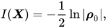
where is the correlation matrix constructed from .[22]

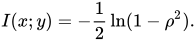
In the bivariate case the expression for the mutual information is:
Joint normality
Normally distributed and independent
If and are normally distributed and independent, this implies they are "jointly normally distributed", i.e., the pair must have multivariate normal distribution. However, a pair of jointly normally distributed variables need not be independent (would only be so if uncorrelated, ).


Two normally distributed random variables need not be jointly bivariate normal
The fact that two random variables and both have a normal distribution does not imply that the pair has a joint normal distribution. A simple example is one in which has a normal distribution with expected value 0 and variance 1, and if and if , where . There are similar counterexamples for more than two random variables. In general, they sum to a mixture model.[citation needed]


Correlations and independence
In general, random variables may be uncorrelated but statistically dependent. But if a random vector has a multivariate normal distribution then any two or more of its components that are uncorrelated are independent. This implies that any two or more of its components that are pairwise independent are independent. But, as pointed out just above, it is not true that two random variables that are (separately, marginally) normally distributed and uncorrelated are independent.
Conditional distributions
If N-dimensional x is partitioned as follows

and accordingly μ and Σ are partitioned as follows


then the distribution of x1 conditional on x2 = a is multivariate normal[23] (x1 | x2 = a) ~ N(μ, Σ) where

and covariance matrix

Here is the generalized inverse of . The matrix is the Schur complement of Σ22 in Σ. That is, the equation above is equivalent to inverting the overall covariance matrix, dropping the rows and columns corresponding to the variables being conditioned upon, and inverting back to get the conditional covariance matrix.


Note that knowing that x2 = a alters the variance, though the new variance does not depend on the specific value of a; perhaps more surprisingly, the mean is shifted by ; compare this with the situation of not knowing the value of a, in which case x1 would have distribution .

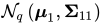
An interesting fact derived in order to prove this result, is that the random vectors and are independent.


The matrix Σ12Σ22−1 is known as the matrix of regression coefficients.
Bivariate case
In the bivariate case where x is partitioned into and , the conditional distribution of given is[25]



where is the correlation coefficient between and .

Bivariate conditional expectation
In the general case

The conditional expectation of X1 given X2 is:

Proof: the result is obtained by taking the expectation of the conditional distribution above.

In the centered case with unit variances

The conditional expectation of X1 given X2 is

and the conditional variance is

thus the conditional variance does not depend on x2.
The conditional expectation of X1 given that X2 is smaller/bigger than z is:[26]: 367
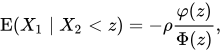
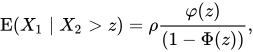
where the final ratio here is called the inverse Mills ratio.
Proof: the last two results are obtained using the result , so that
- and then using the properties of the expectation of a truncated normal distribution.

Marginal distributions
To obtain the marginal distribution over a subset of multivariate normal random variables, one only needs to drop the irrelevant variables (the variables that one wants to marginalize out) from the mean vector and the covariance matrix. The proof for this follows from the definitions of multivariate normal distributions and linear algebra.[27]
Example
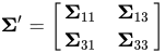
Let X = [X1, X2, X3] be multivariate normal random variables with mean vector μ = [μ1, μ2, μ3] and covariance matrix Σ (standard parametrization for multivariate normal distributions). Then the joint distribution of X′ = [X1, X3] is multivariate normal with mean vector μ′ = [μ1, μ3] and covariance matrix .
Affine transformation
If Y = c + BX is an affine transformation of where c is an vector of constants and B is a constant matrix, then Y has a multivariate normal distribution with expected value c + Bμ and variance BΣBT i.e., . In particular, any subset of the Xi has a marginal distribution that is also multivariate normal. To see this, consider the following example: to extract the subset (X1, X2, X4)T, use



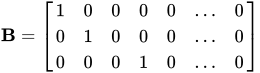
which extracts the desired elements directly.
Another corollary is that the distribution of Z = b · X, where b is a constant vector with the same number of elements as X and the dot indicates the dot product, is univariate Gaussian with . This result follows by using


Observe how the positive-definiteness of Σ implies that the variance of the dot product must be positive.
An affine transformation of X such as 2X is not the same as the sum of two independent realisations of X.
Geometric interpretation
The equidensity contours of a non-singular multivariate normal distribution are ellipsoids (i.e. affine transformations of hyperspheres) centered at the mean.[28] Hence the multivariate normal distribution is an example of the class of elliptical distributions. The directions of the principal axes of the ellipsoids are given by the eigenvectors of the covariance matrix . The squared relative lengths of the principal axes are given by the corresponding eigenvalues.
If Σ = UΛUT = UΛ1/2(UΛ1/2)T is an eigendecomposition where the columns of U are unit eigenvectors and Λ is a diagonal matrix of the eigenvalues, then we have

Moreover, U can be chosen to be a rotation matrix, as inverting an axis does not have any effect on N(0, Λ), but inverting a column changes the sign of U's determinant. The distribution N(μ, Σ) is in effect N(0, I) scaled by Λ1/2, rotated by U and translated by μ.
Conversely, any choice of μ, full rank matrix U, and positive diagonal entries Λi yields a non-singular multivariate normal distribution. If any Λi is zero and U is square, the resulting covariance matrix UΛUT is singular. Geometrically this means that every contour ellipsoid is infinitely thin and has zero volume in n-dimensional space, as at least one of the principal axes has length of zero; this is the degenerate case.
"The radius around the true mean in a bivariate normal random variable, re-written in polar coordinates (radius and angle), follows a Hoyt distribution."[29]
In one dimension the probability of finding a sample of the normal distribution in the interval is approximately 68.27%, but in higher dimensions the probability of finding a sample in the region of the standard deviation ellipse is lower.[30]

| Dimensionality | Probability |
|---|---|
| 1 | 0.6827 |
| 2 | 0.3935 |
| 3 | 0.1987 |
| 4 | 0.0902 |
| 5 | 0.0374 |
| 6 | 0.0144 |
| 7 | 0.0052 |
| 8 | 0.0018 |
| 9 | 0.0006 |
| 10 | 0.0002 |
Statistical inference
Parameter estimation
The derivation of the maximum-likelihood estimator of the covariance matrix of a multivariate normal distribution is straightforward.
In short, the probability density function (pdf) of a multivariate normal is

and the ML estimator of the covariance matrix from a sample of n observations is [31]
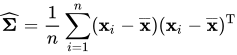
which is simply the sample covariance matrix. This is a biased estimator whose expectation is
![{\displaystyle E\left[{\widehat {\boldsymbol {\Sigma }}}\right]={\frac {n-1}{n}}{\boldsymbol {\Sigma }}.}](https://wikimedia.org/api/rest_v1/media/math/render/svg/12908e94489d8fcdd7c2aa360d3ce85c26bc611a)
An unbiased sample covariance is
- (matrix form; is the identity matrix, J is a matrix of ones; the term in parentheses is thus the centering matrix)
![{\displaystyle {\widehat {\boldsymbol {\Sigma }}}={\frac {1}{n-1}}\sum _{i=1}^{n}(\mathbf {x} _{i}-{\overline {\mathbf {x} }})(\mathbf {x} _{i}-{\overline {\mathbf {x} }})^{\rm {T}}={\frac {1}{n-1}}\left[X'\left(I-{\frac {1}{n}}\cdot J\right)X\right]}](https://wikimedia.org/api/rest_v1/media/math/render/svg/b483843b0f64ecbfea751011ef0ab8e61c7f0dcc)


The Fisher information matrix for estimating the parameters of a multivariate normal distribution has a closed form expression. This can be used, for example, to compute the Cramér–Rao bound for parameter estimation in this setting. See Fisher information for more details.
Bayesian inference
In Bayesian statistics, the conjugate prior of the mean vector is another multivariate normal distribution, and the conjugate prior of the covariance matrix is an inverse-Wishart distribution . Suppose then that n observations have been made


and that a conjugate prior has been assigned, where

where

and

Then[31]

where

Multivariate normality tests
Multivariate normality tests check a given set of data for similarity to the multivariate normal distribution. The null hypothesis is that the data set is similar to the normal distribution, therefore a sufficiently small p-value indicates non-normal data. Multivariate normality tests include the Cox–Small test[32] and Smith and Jain's adaptation[33] of the Friedman–Rafsky test created by Larry Rafsky and Jerome Friedman.[34]
Mardia's test
Mardia's test[35] is based on multivariate extensions of skewness and kurtosis measures. For a sample {x1, ..., xn} of k-dimensional vectors we compute
![{\displaystyle {\begin{aligned}&{\widehat {\boldsymbol {\Sigma }}}={1 \over n}\sum _{j=1}^{n}\left(\mathbf {x} _{j}-{\bar {\mathbf {x} }}\right)\left(\mathbf {x} _{j}-{\bar {\mathbf {x} }}\right)^{\mathrm {T} }\\&A={1 \over 6n}\sum _{i=1}^{n}\sum _{j=1}^{n}\left[(\mathbf {x} _{i}-{\bar {\mathbf {x} }})^{\mathrm {T} }\;{\widehat {\boldsymbol {\Sigma }}}^{-1}(\mathbf {x} _{j}-{\bar {\mathbf {x} }})\right]^{3}\\&B={\sqrt {\frac {n}{8k(k+2)}}}\left\{{1 \over n}\sum _{i=1}^{n}\left[(\mathbf {x} _{i}-{\bar {\mathbf {x} }})^{\mathrm {T} }\;{\widehat {\boldsymbol {\Sigma }}}^{-1}(\mathbf {x} _{i}-{\bar {\mathbf {x} }})\right]^{2}-k(k+2)\right\}\end{aligned}}}](https://wikimedia.org/api/rest_v1/media/math/render/svg/2d6fcd342cc6e6df3c6fcd10852c7908e248829d)
Under the null hypothesis of multivariate normality, the statistic A will have approximately a chi-squared distribution with 1/6⋅k(k + 1)(k + 2) degrees of freedom, and B will be approximately standard normal N(0,1).
Mardia's kurtosis statistic is skewed and converges very slowly to the limiting normal distribution. For medium size samples , the parameters of the asymptotic distribution of the kurtosis statistic are modified[36] For small sample tests () empirical critical values are used. Tables of critical values for both statistics are given by Rencher[37] for k = 2, 3, 4.


Mardia's tests are affine invariant but not consistent. For example, the multivariate skewness test is not consistent against symmetric non-normal alternatives.[38]
BHEP test
The BHEP test[39] computes the norm of the difference between the empirical characteristic function and the theoretical characteristic function of the normal distribution. Calculation of the norm is performed in the L2(μ) space of square-integrable functions with respect to the Gaussian weighting function . The test statistic is


The limiting distribution of this test statistic is a weighted sum of chi-squared random variables.[39]
A detailed survey of these and other test procedures is available.[40]
Computational methods
Drawing values from the distribution
A widely used method for drawing (sampling) a random vector x from the N-dimensional multivariate normal distribution with mean vector μ and covariance matrix Σ works as follows:[41]
- Find any real matrix A such that AAT = Σ. When Σ is positive-definite, the Cholesky decomposition is typically used because it is widely available, computationally efficient, and well known. If a rank-revealing (pivoted) Cholesky decomposition such as LAPACK's dpstrf() is available, it can be used in the general positive-semidefinite case as well. A slower general alternative is to use the matrix A = UΛ1/2 obtained from a spectral decomposition Σ = UΛU−1 of Σ.
- Let z = (z1, ..., zN)T be a vector whose components are N independent standard normal variates (which can be generated, for example, by using the Box–Muller transform).
- Let x be μ + Az. This has the desired distribution due to the affine transformation property.
See also
- Chi distribution, the pdf of the 2-norm (Euclidean norm or vector length) of a multivariate normally distributed vector (uncorrelated and zero centered).
- Rayleigh distribution, the pdf of the vector length of a bivariate normally distributed vector (uncorrelated and zero centered)
- Rice distribution, the pdf of the vector length of a bivariate normally distributed vector (uncorrelated and non-centered)
- Hoyt distribution, the pdf of the vector length of a bivariate normally distributed vector (correlated and centered)
- Complex normal distribution, an application of bivariate normal distribution
- Copula, for the definition of the Gaussian or normal copula model.
- Multivariate t-distribution, which is another widely used spherically symmetric multivariate distribution.
- Multivariate stable distribution extension of the multivariate normal distribution, when the index (exponent in the characteristic function) is between zero and two.
- Mahalanobis distance
- Wishart distribution
- Matrix normal distribution
References
- 1 2 3 Lapidoth, Amos (2009). A Foundation in Digital Communication. Cambridge University Press. ISBN 978-0-521-19395-5.
- ↑ Gut, Allan (2009). An Intermediate Course in Probability. Springer. ISBN 978-1-441-90161-3.
- ↑ Kac, M. (1939). "On a characterization of the normal distribution". American Journal of Mathematics. 61 (3): 726–728. doi:10.2307/2371328. JSTOR 2371328.
- ↑ Sinz, Fabian; Gerwinn, Sebastian; Bethge, Matthias (2009). "Characterization of the p-generalized normal distribution". Journal of Multivariate Analysis. 100 (5): 817–820. doi:10.1016/j.jmva.2008.07.006.
- ↑ Simon J.D. Prince(June 2012). Computer Vision: Models, Learning, and Inference Archived 2020-10-28 at the Wayback Machine. Cambridge University Press. 3.7:"Multivariate normal distribution".
- ↑ Kim, M. G. (2000). "Multivariate outliers and decompositions of Mahalanobis distance". Communications in Statistics – Theory and Methods. 29 (7): 1511–1526. doi:10.1080/03610920008832559.
- ↑ Hamedani, G. G.; Tata, M. N. (1975). "On the determination of the bivariate normal distribution from distributions of linear combinations of the variables". The American Mathematical Monthly. 82 (9): 913–915. doi:10.2307/2318494. JSTOR 2318494.
- ↑ Wyatt, John (November 26, 2008). "Linear least mean-squared error estimation" (PDF). Lecture notes course on applied probability. Archived from the original (PDF) on October 10, 2015. Retrieved 23 January 2012.
- ↑ "linear algebra - Mapping between affine coordinate function". Mathematics Stack Exchange. Retrieved 2022-06-24.
- ↑ Rao, C. R. (1973). Linear Statistical Inference and Its Applications. New York: Wiley. pp. 527–528. ISBN 0-471-70823-2.
- 1 2 Botev, Z. I. (2016). "The normal law under linear restrictions: simulation and estimation via minimax tilting". Journal of the Royal Statistical Society, Series B. 79: 125–148. arXiv:1603.04166. Bibcode:2016arXiv160304166B. doi:10.1111/rssb.12162. S2CID 88515228.
- ↑ Genz, Alan (2009). Computation of Multivariate Normal and t Probabilities. Springer. ISBN 978-3-642-01689-9.
- 1 2 Bensimhoun Michael, N-Dimensional Cumulative Function, And Other Useful Facts About Gaussians and Normal Densities (2006)
- ↑ Siotani, Minoru (1964). "Tolerance regions for a multivariate normal population" (PDF). Annals of the Institute of Statistical Mathematics. 16 (1): 135–153. doi:10.1007/BF02868568. S2CID 123269490.
- 1 2 Botev, Z. I.; Mandjes, M.; Ridder, A. (6–9 December 2015). "Tail distribution of the maximum of correlated Gaussian random variables". 2015 Winter Simulation Conference (WSC). Huntington Beach, Calif., USA: IEEE. pp. 633–642. doi:10.1109/WSC.2015.7408202. hdl:10419/130486. ISBN 978-1-4673-9743-8.
- ↑ Adler, R. J.; Blanchet, J.; Liu, J. (7–10 Dec 2008). "Efficient simulation for tail probabilities of Gaussian random fields". 2008 Winter Simulation Conference (WSC). Miami, Fla., USA: IEEE. pp. 328–336. doi:10.1109/WSC.2008.4736085. ISBN 978-1-4244-2707-9.
- ↑ Hernandez-Stumpfhauser, Daniel; Breidt, F. Jay; van der Woerd, Mark J. (2017). "The General Projected Normal Distribution of Arbitrary Dimension: Modeling and Bayesian Inference". Bayesian Analysis. 12 (1): 113–133. doi:10.1214/15-BA989.
- ↑ Tong, T. (2010) Multiple Linear Regression : MLE and Its Distributional Results Archived 2013-06-16 at WebCite, Lecture Notes
- ↑ Gokhale, DV; Ahmed, NA; Res, BC; Piscataway, NJ (May 1989). "Entropy Expressions and Their Estimators for Multivariate Distributions". IEEE Transactions on Information Theory. 35 (3): 688–692. doi:10.1109/18.30996.
- ↑ Duchi, J. Derivations for Linear Algebra and Optimization (PDF) (Thesis). p. 13. Archived from the original (PDF) on 2020-07-25. Retrieved 2020-08-12.
- ↑ Proof: Mutual information of the multivariate normal distribution
- ↑ MacKay, David J. C. (2003-10-06). Information Theory, Inference and Learning Algorithms (Illustrated ed.). Cambridge: Cambridge University Press. ISBN 978-0-521-64298-9.
- ↑ Holt, W.; Nguyen, D. (2023). Essential Aspects of Bayesian Data Imputation (Thesis). SSRN 4494314.
- ↑ Eaton, Morris L. (1983). Multivariate Statistics: a Vector Space Approach. John Wiley and Sons. pp. 116–117. ISBN 978-0-471-02776-8.
- ↑ Jensen, J (2000). Statistics for Petroleum Engineers and Geoscientists. Amsterdam: Elsevier. p. 207. ISBN 0-444-50552-0.
- ↑ Maddala, G. S. (1983). Limited Dependent and Qualitative Variables in Econometrics. Cambridge University Press. ISBN 0-521-33825-5.
- ↑ An algebraic computation of the marginal distribution is shown here http://fourier.eng.hmc.edu/e161/lectures/gaussianprocess/node7.html Archived 2010-01-17 at the Wayback Machine. A much shorter proof is outlined here https://math.stackexchange.com/a/3832137
- ↑ Nikolaus Hansen (2016). "The CMA Evolution Strategy: A Tutorial" (PDF). arXiv:1604.00772. Bibcode:2016arXiv160400772H. Archived from the original (PDF) on 2010-03-31. Retrieved 2012-01-07.
- ↑ Daniel Wollschlaeger. "The Hoyt Distribution (Documentation for R package 'shotGroups' version 0.6.2)".[permanent dead link]
- ↑ Wang, Bin; Shi, Wenzhong; Miao, Zelang (2015-03-13). Rocchini, Duccio (ed.). "Confidence Analysis of Standard Deviational Ellipse and Its Extension into Higher Dimensional Euclidean Space". PLOS ONE. 10 (3) e0118537. Bibcode:2015PLoSO..1018537W. doi:10.1371/journal.pone.0118537. ISSN 1932-6203. PMC 4358977. PMID 25769048.
- 1 2 Holt, W.; Nguyen, D. (2023). Introduction to Bayesian Data Imputation (Thesis). SSRN 4494314.
- ↑ Cox, D. R.; Small, N. J. H. (1978). "Testing multivariate normality". Biometrika. 65 (2): 263. doi:10.1093/biomet/65.2.263.
- ↑ Smith, S. P.; Jain, A. K. (1988). "A test to determine the multivariate normality of a data set". IEEE Transactions on Pattern Analysis and Machine Intelligence. 10 (5): 757. doi:10.1109/34.6789.
- ↑ Friedman, J. H.; Rafsky, L. C. (1979). "Multivariate Generalizations of the Wald–Wolfowitz and Smirnov Two-Sample Tests". The Annals of Statistics. 7 (4): 697. doi:10.1214/aos/1176344722.
- ↑ Mardia, K. V. (1970). "Measures of multivariate skewness and kurtosis with applications". Biometrika. 57 (3): 519–530. doi:10.1093/biomet/57.3.519.
- ↑ Rencher (1995), pages 112–113.
- ↑ Rencher (1995), pages 493–495.
- ↑ Baringhaus, L.; Henze, N. (1991). "Limit distributions for measures of multivariate skewness and kurtosis based on projections". Journal of Multivariate Analysis. 38: 51–69. doi:10.1016/0047-259X(91)90031-V.
- 1 2 Baringhaus, L.; Henze, N. (1988). "A consistent test for multivariate normality based on the empirical characteristic function". Metrika. 35 (1): 339–348. doi:10.1007/BF02613322. S2CID 122362448.
- ↑ Henze, Norbert (2002). "Invariant tests for multivariate normality: a critical review". Statistical Papers. 43 (4): 467–506. doi:10.1007/s00362-002-0119-6. S2CID 122934510.
- ↑ Gentle, J. E. (2009). Computational Statistics. Statistics and Computing. New York: Springer. pp. 315–316. doi:10.1007/978-0-387-98144-4. ISBN 978-0-387-98143-7.
Literature
- Rencher, A.C. (1995). Methods of Multivariate Analysis. New York: Wiley.
- Tong, Y. L. (1990). The multivariate normal distribution. Springer Series in Statistics. New York: Springer-Verlag. doi:10.1007/978-1-4613-9655-0. ISBN 978-1-4613-9657-4. S2CID 120348131.


| |||||||||||||||||||||||||||
| |||||||||||||||||||||||||||
| |||||||||||||||||||||||||||
| |||||||||||||||||||||||||||
| |||||||||||||||||||||||||||
| |||||||||||||||||||||||||||
| |||||||||||||||||||||||||||


