TÄNA AJALOOS, 11. juuli ⟩ Avati Tallinna teletorn

In mathematics, the Neumann (or second-type) boundary condition is a type of boundary condition, named after Carl Neumann.^[1] When imposed on an ordinary or a partial differential equation, the condition specifies the values of the derivative applied at the boundary of the domain.

It is possible to describe the problem using other boundary conditions: a Dirichlet boundary condition specifies the values of the solution itself (as opposed to its derivative) on the boundary, whereas the Cauchy boundary condition, mixed boundary condition and Robin boundary condition are all different types of combinations of the Neumann and Dirichlet boundary conditions.

Examples

ODE

For an ordinary differential equation, for instance,

y''+y=0,

the Neumann boundary conditions on the interval $[a, b]$ take the form

y'(a)=\alpha ,\quad y'(b)=\beta ,

where $α$ and $β$ are given numbers.

PDE

For a partial differential equation, for instance,

\nabla ^{2}y+y=0,

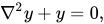
where $\nabla 2$ denotes the Laplace operator, the Neumann boundary conditions on a domain $Ω \subset R n$ take the form

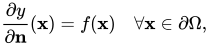
{\frac {\partial y}{\partial \mathbf {n} }}(\mathbf {x} )=f(\mathbf {x} )\quad \forall \mathbf {x} \in \partial \Omega ,

where the left hand side is called the normal derivative, and is defined as the inner product of the gradient vector of $y (x)$ , $\nabla y (x)$ , and the (typically exterior) unit normal to the boundary $\partialΩ$

{\frac {\partial y}{\partial \mathbf {n} }}(\mathbf {x} )=\nabla y(\mathbf {x} )\cdot \mathbf {\hat {n}} (\mathbf {x} ),

and $f$ is a given scalar function.

It becomes clear that the boundary must be sufficiently smooth such that the normal derivative can exist, since, for example, at corner points on the boundary the normal vector is not well defined.

Applications

The following applications involve the use of Neumann boundary conditions:

In thermodynamics, a prescribed heat flux from a surface would serve as boundary condition. For example, a perfect insulator would have no flux while an electrical component may be dissipating at a known power.
In magnetostatics, the magnetic field intensity can be prescribed as a boundary condition in order to find the magnetic flux density distribution in a magnet array in space, for example in a permanent magnet motor. Since the problems in magnetostatics involve solving Laplace's equation or Poisson's equation for the magnetic scalar potential, the boundary condition is a Neumann condition.
In spatial ecology, a Neumann boundary condition on a reaction–diffusion system, such as Fisher's equation, can be interpreted as a reflecting boundary, such that all individuals encountering $\partialΩ$ are reflected back onto $Ω$ .^[2]

References

↑ Cheng, A. H.-D.; Cheng, D. T. (2005). "Heritage and early history of the boundary element method". Engineering Analysis with Boundary Elements. 29 (3): 268. doi:10.1016/j.enganabound.2004.12.001.
↑ Cantrell, Robert Stephen; Cosner, Chris (2003). Spatial Ecology via Reaction–Diffusion Equations. Wiley. pp. 30–31. ISBN 0-471-49301-5.